Google Data Analysis Capstone Project

Cyclistic RideShare Case Study

(SQL and Tableau)

Daniel Morgan

Case Summary:

Cyclistic is a bike share company with a fleet of bicycles that are geotracked and locked into a network of stations across Chicago. Cyclistic has three pricing plans: single-ride passes, full-day passes, and annual memberships. Customers who purchase single-ride or full-day passes are referred to as casual riders. Customers who purchase annual memberships are annual members.

The main focus of this case is to explore ride data in the hopes of discovering differences in the way annual members and casual riders use Cyclistic’s bikes.

These insights will then be used to design marketing strategies aimed at converting casual riders into much more profitable annual members.

Findings:

(Please continue reading for detailed analysis process and documentation)

The data suggests that Cyclistic users fall into two categories: Chicago locals who use the bikeshare mainly for daily transportation purposes, and riders who use the service for Chicago tourism activities - largely on the weekends during the warmer months of the year.

Therefore, it is my recommendation to proceed with a two pronged marketing strategy with specific focuses for tourists and locals.

For the tourism side of the marketing, my recommendation is to highlight the value of repeat trips and also consider an alternative “Weekend Membership” or multiple day pass offering to entice visitors to spend more with the service. The data suggests tourism focused media (e.g. visitors guides, weekend guides, specific event guides) emphasizing weekends in the spring and summer months will be the most effective, with a message promoting value and the “sightseeing advantages of exploring the city by bike” for example.

For the marketing effort aimed at Chicago locals, the data suggests focusing on added convenience and value through use of the service. It is recommended to time the marketing in the spring, when the value proposition is the greatest, although further research into membership sign up timing could provide valuable insights. Also, further research into concerns locals may have about using the service (e.g. safety, stress, etc.) could help the marketing effort to overcome the most common objections to membership. I recommend geographically focused marketing near the most used stations, as well as further research into why these stations are so popular in hopes of developing other stations and their surrounding population.

Overall, this research has been insightful and beneficial and I feel optimistic for the continued growth and success of Cyclistic.

Detailed Analysis Process:

Phase 1: Ask

1. Identify The Business Task:

Discover ways in which annual members and casual riders use Cyclistic bikes differently, use these insights to guide a marketing campaign aimed at converting casual riders into annual members.

Produce a report with the following deliverables:

1. A clear statement of the business task

2. A description of all data sources used

3. Documentation of any cleaning or manipulation of data

4. A summary of your analysis

5. Supporting visualizations and key findings

6. Your top three recommendations based on your analysis

2. Consider key stakeholders:

Cyclistic Executive Team

Lily Moreno - Director of Marketing

Cyclistic Marketing Analytics Team

Phase 2: Prepare

1. General data set information:

The data has been made available by Motivate International Inc. (Divvy), (which for the purposes of this exercise has been renamed Cyclistic) under this license. It is available here. The data is in .csv files and arranged by month. The data does not appear to have issues with bias or credibility, however data-privacy issues prohibit use of riders’ personally identifiable information, so it will not be possible to connect pass purchases to credit card numbers to determine if casual riders live in the Cyclistic service area or if they have purchased multiple single passes - information that would be valuable within the scope of this assignment. I will be using the most current 12 months, Aug. 2021 - July 2022. The data is in 12 spreadsheets, by month, and in total is over 1 GB in size. Because of this large size I will be using SQL in BIGQUERY to do all the work with the data and Tableau for visualizations.

I begin by uploading all twelve files into google cloud and loading them into BIGQUERY. Next, merge all the tables:

CREATE TABLE `cyclistic_case_study.aggregate_table`
(ride_id STRING, rideable_type STRING, started_at TIMESTAMP, ended_at TIMESTAMP, start_lat FLOAT64, start_lng FLOAT64, end_lat FLOAT64, end_lng FLOAT64, member_casual STRING, start_station_name STRING, end_station_name STRING);
INSERT INTO `cyclistic_case_study.aggregate_table` (ride_id, rideable_type, started_at, ended_at, start_lat, start_lng, end_lat, end_lng, member_casual, start_station_name, end_station_name)
(SELECT
ride_id, rideable_type, started_at, ended_at, start_lat, start_lng, end_lat, end_lng, member_casual, start_station_name, end_station_name
FROM
`cyclistic_case_study.aug21data`
UNION DISTINCT
SELECT
ride_id, rideable_type, started_at, ended_at, start_lat, start_lng, end_lat, end_lng, member_casual, start_station_name, end_station_name
FROM
`cyclistic_case_study.sep21data`
UNION DISTINCT
SELECT
ride_id, rideable_type, started_at, ended_at, start_lat, start_lng, end_lat, end_lng, member_casual, start_station_name, end_station_name
FROM
`cyclistic_case_study.oct21data`
UNION DISTINCT
SELECT
ride_id, rideable_type, started_at, ended_at, start_lat, start_lng, end_lat, end_lng, member_casual, start_station_name, end_station_name
FROM
`cyclistic_case_study.nov21data`
UNION DISTINCT
SELECT
ride_id, rideable_type, started_at, ended_at, start_lat, start_lng, end_lat, end_lng, member_casual, start_station_name, end_station_name
FROM
`cyclistic_case_study.dec21data`
UNION DISTINCT
SELECT
ride_id, rideable_type, started_at, ended_at, start_lat, start_lng, end_lat, end_lng, member_casual, start_station_name, end_station_name
FROM
`cyclistic_case_study.jan22data`
UNION DISTINCT
SELECT
ride_id, rideable_type, started_at, ended_at, start_lat, start_lng, end_lat, end_lng, member_casual, start_station_name, end_station_name
FROM
`cyclistic_case_study.feb22data`
UNION DISTINCT
SELECT
ride_id, rideable_type, started_at, ended_at, start_lat, start_lng, end_lat, end_lng, member_casual, start_station_name, end_station_name
FROM
`cyclistic_case_study.mar22data`
UNION DISTINCT
SELECT
ride_id, rideable_type, started_at, ended_at, start_lat, start_lng, end_lat, end_lng, member_casual, start_station_name, end_station_name
FROM
`cyclistic_case_study.apr22data`
UNION DISTINCT
SELECT
ride_id, rideable_type, started_at, ended_at, start_lat, start_lng, end_lat, end_lng, member_casual, start_station_name, end_station_name
FROM
`cyclistic_case_study.may22data`
UNION DISTINCT
SELECT
ride_id, rideable_type, started_at, ended_at, start_lat, start_lng, end_lat, end_lng, member_casual, start_station_name, end_station_name
FROM
`cyclistic_case_study.jun22data`
UNION DISTINCT
SELECT
ride_id, rideable_type, started_at, ended_at, start_lat, start_lng, end_lat, end_lng, member_casual, start_station_name, end_station_name
FROM
`cyclistic_case_study.jul22data`);

Phase 3: Process

1. Data Cleaning Process and Documentation:

Total record count = 5,901,463 :

SELECT COUNT (*)
FROM `cyclistic_case_study.aggregate_table`;

Add day of week column:

ALTER TABLE `cyclistic_case_study.aggregate_table`
ADD COLUMN day_of_week STRING;

UPDATE `cyclistic_case_study.aggregate_table`
SET day_of_week = FORMAT_DATE('%A', started_at)
WHERE TRUE;

Add ride time column:

ALTER TABLE `cyclistic_case_study.aggregate_table`
ADD COLUMN ride_time INT64;

UPDATE `cyclistic_case_study.aggregate_table`
SET ride_time = TIMESTAMP_DIFF(ended_at , started_at, SECOND)
WHERE TRUE;

Count duplicate ride id’s (there were zero):

SELECT COUNT (DISTINCT (ride_id)) AS ride_id_count
FROM `cyclistic_case_study.aggregate_table`;

Check for alternate spelling/entries of membership and ride types (there were zero):

SELECT rideable_type,
member_casual
FROM `cyclistic_case_study.aggregate_table`
GROUP BY rideable_type, member_casual;

Check for instances where end time is before start time, there are 149 instances of this:

SELECT COUNT(ride_time)
FROM `central-surf-345019.cyclistic_case_study.aggregate_table`
WHERE ended_at < started_at;

Check for NULL values in the latitude and longitude columns, there are 5590:

SELECT COUNT(*)
FROM `central-surf-345019.cyclistic_case_study.aggregate_table`
WHERE start_lat IS NULL
OR
start_lng IS NULL
OR
end_lat IS NULL
OR
end_lng IS NULL;

Check for NULL values in the start or end station name columns, there are 1,272,233 this represents a substantial portion (21%) of the 5,901,463 total entries in this data set:

SELECT COUNT(*)
FROM `central-surf-345019.cyclistic_case_study.aggregate_table`
WHERE start_station_name IS NULL
OR
end_station_name IS NULL;

Because of the large percentage of NULL values, I am reluctant to just delete all these records, especially since they otherwise appear to be normal rides. In a real world situation I would inquire for the reason why a ride could begin or end without a station being logged. Also, upon further examination, it appears that a null value may be entered if the latitude or longitude figure is off by as little as .002° from the defined coordinates of each station (see: Hastings WH 2 entries for evidence). For this reason and the purpose of this exercise I will keep these entries in order to have more data to work with.

I will now continue to investigate these columns for entries that may not be relevant to the study.

Next, I check for distinct start station and end station names:

SELECT DISTINCT start_station_name, end_station_name
FROM `central-surf-345019.cyclistic_case_study.aggregate_table`;

I notice most of the stations are named after intersections, for example: “LaSalle St & Adams St”, so I write a query to filter results that include the ‘&’ symbol to reduce the number of stations I have to look through to see if there are any unusual names e.g. ‘service’ or ‘test’:

SELECT DISTINCT start_station_name, end_station_name
FROM `central-surf-345019.cyclistic_case_study.aggregate_table`
WHERE NOT (start_station_name LIKE '%&%' OR end_station_name LIKE '%&%');

There were several entries that required further investigation, out of those, there are 1800 entries going to or coming from 2132 W Hubbard in Chicago, which a quick maps search shows as the Divvy service warehouse, as service stops are not legitimate trips I will be deleting these entries. Also, there are 2 entries listed as DIVVY CASSETTE REPAIR MOBILE STATION, and 1 entry labeled ‘Pawel Bialowas - Test- PBSC charging station’, these will also need to be deleted.

SELECT *
FROM `central-surf-345019.cyclistic_case_study.aggregate_table`
WHERE start_station_name LIKE ('%WH%') OR end_station_name LIKE ('%WH%');

Create Backup table (Same aggregate query as before, now named `central-surf-345019.cyclistic_case_study.aggregate_table_backup`)

Delete the records that are not relevant to analysis:

DELETE FROM `cyclistic_case_study.aggregate_table`
WHERE ended_at < started_at;

DELETE FROM `cyclistic_case_study.aggregate_table`
WHERE start_lat IS NULL
OR
start_lng IS NULL
OR
end_lat IS NULL
OR
end_lng IS NULL;

DELETE FROM `cyclistic_case_study.aggregate_table`
WHERE start_station_name LIKE ('%2132 W Hubbard%') OR end_station_name LIKE ('%2132 W Hubbard%')
OR start_station_name LIKE ('%DIVVY%') OR end_station_name LIKE ('%DIVVY%')
OR start_station_name LIKE ('%Pawel%') OR end_station_name LIKE ('%Pawel%');

Double check the new total record count = 5,893,922

SELECT COUNT (*)
FROM `cyclistic_case_study.aggregate_table`;

Phase 4: Analyze

1. Analysis Process and Documentation:

SQL:

Total Rides by Member Type

SELECT member_casual,
COUNT(ride_id) AS total_rides
FROM `cyclistic_case_study.aggregate_table`
GROUP BY member_casual
ORDER BY member_casual;

Average Ride Time per Membership Type

SELECT member_casual,
AVG(ride_time) AS average_ride_time,
FROM `cyclistic_case_study.aggregate_table`
GROUP BY member_casual
ORDER BY member_casual;

Count of rideable type and average time by member and bike type:

SELECT member_casual, rideable_type,
AVG(ride_time) AS average_ride_time,
COUNT (rideable_type) AS bike_totals,
day_of_week
FROM `cyclistic_case_study.aggregate_table`
GROUP BY rideable_type, member_casual
ORDER BY member_casual;

Ride Count and Average Ride Time by Membership Type and Day of Week

SELECT member_casual, day_of_week,
AVG(ride_time) AS average_ride_time,
COUNT(started_at) AS Number_of_Rides
FROM `cyclistic_case_study.aggregate_table`
GROUP BY member_casual, day_of_week
ORDER BY member_casual;

Count of rideable type by month:

SELECT member_casual, rideable_type,
EXTRACT(MONTH from started_at) AS month,
COUNT (rideable_type) AS bike_totals,
FROM `cyclistic_case_study.aggregate_table`
GROUP BY rideable_type, member_casual, month
ORDER BY month;

Average ride time and monthly total by membership type:

SELECT member_casual,
EXTRACT(MONTH from started_at) AS month,
AVG(ride_time) AS average_ride_time,
COUNT (started_at) AS monthly_total,
FROM `cyclistic_case_study.aggregate_table`
GROUP BY member_casual, month
ORDER BY month;

Count avg ride time and number of rides by day of week and month and membership and ride type:

SELECT member_casual, rideable_type,
EXTRACT(MONTH from started_at) AS month,
AVG(ride_time) AS average_ride_time,
COUNT (rideable_type) AS bike_totals,day_of_week,
FROM `cyclistic_case_study.aggregate_table`
GROUP BY rideable_type, member_casual, day_of_week, month
ORDER BY month;

Next, I want to look at the most used stations, so I will pull that data to create a spreadsheet for analysis.

Count top 20 starting and ending stations for casual and member riders:

SELECT start_station_name,
COUNT(start_station_name) AS top_casual_starts,
FROM `cyclistic_case_study.aggregate_table`
WHERE member_casual = 'casual'
GROUP BY start_station_name, member_casual
ORDER BY top_casual_starts DESC
LIMIT 20;

SELECT member_casual, end_station_name,
COUNT(end_station_name) AS top_casual_ends,
FROM `cyclistic_case_study.aggregate_table`
WHERE member_casual = 'casual'
GROUP BY end_station_name, member_casual
ORDER BY top_casual_ends DESC
LIMIT 20;

SELECT member_casual, start_station_name,
COUNT(start_station_name) AS top_member_starts,
FROM `cyclistic_case_study.aggregate_table`
WHERE member_casual = 'member'
GROUP BY start_station_name, member_casual
ORDER BY top_member_starts DESC
LIMIT 20;

SELECT member_casual, end_station_name,
COUNT(end_station_name) AS top_member_ends,
FROM `cyclistic_case_study.aggregate_table`
WHERE member_casual = 'member'
GROUP BY end_station_name, member_casual
ORDER BY top_member_ends DESC
LIMIT 20;

Looking at the most used stations, it looks like casual riders visit more stations that could be considered “touristy” than members, I wonder if the most used member stations change to be more touristy on the weekends?

Count top 30 starting and ending weekend stations for member riders to compile top 20 list:

SELECT member_casual, start_station_name,
COUNT(start_station_name) AS top_member_weekend_starts,
FROM `cyclistic_case_study.aggregate_table`
WHERE member_casual = 'member'
AND day_of_week = "Saturday"
GROUP BY start_station_name, member_casual
ORDER BY top_member_weekend_starts DESC
LIMIT 30;

SELECT member_casual, start_station_name,
COUNT(start_station_name) AS top_member_weekend_starts,
FROM `cyclistic_case_study.aggregate_table`
WHERE member_casual = 'member'
AND day_of_week = "Sunday"
GROUP BY start_station_name, member_casual
ORDER BY top_member_weekend_starts DESC
LIMIT 30;

SELECT member_casual, end_station_name,
COUNT(end_station_name) AS top_member_weekend_ends,
FROM `cyclistic_case_study.aggregate_table`
WHERE member_casual = 'member'
AND day_of_week = "Saturday"
GROUP BY end_station_name, member_casual
ORDER BY top_member_weekend_ends DESC
LIMIT 30;

SELECT member_casual, end_station_name,
COUNT(end_station_name) AS top_member_weekend_ends,
FROM `cyclistic_case_study.aggregate_table`
WHERE member_casual = 'member'
AND day_of_week = "Sunday"
GROUP BY end_station_name, member_casual
ORDER BY top_member_weekend_ends DESC
LIMIT 30;

I want to try and look for insights in the provided latitude and longitude information:

Create table with ride distance, named `central-surf-345019.cyclistic_case_study.member_ridetype_day_time_distance` :

SELECT member_casual, rideable_type, day_of_week, ride_time,
ST_DISTANCE(
st_geogpoint(start_lng, start_lat),
st_geogpoint(end_lng, end_lat)
) AS distance_in_meters
FROM `cyclistic_case_study.aggregate_table`
ORDER BY member_casual;

It looks like this distance information is all over the place, I wonder if I can separate round trips and find anything useful in that data?

Count where distance is <15 meters, >16:

SELECT member_casual,
COUNT(distance_in_meters) AS round_trip_rides
FROM `central-surf-345019.cyclistic_case_study.member_ridetype_day_time_distance`
WHERE distance_in_meters <15
GROUP BY member_casual
ORDER BY member_casual;

SELECT member_casual,
AVG(distance_in_meters) AS average_distance
FROM `central-surf-345019.cyclistic_case_study.member_ridetype_day_time_distance`
WHERE distance_in_meters >16
GROUP BY member_casual
ORDER BY member_casual;

Even filtering for round trips based on start and ending location data, it is really not possible to get useful info outside of the most popular stations, which I already have. It would potentially be very beneficial to Cyclistic to examine the actual GPS data of trips and where, specifically, riders are going.

This concludes the SQL portion of the analysis, I now transfer the data from BIGQUERY to Tableau, let’s see what the data shows us!

Phase 5: Share

Tableau:

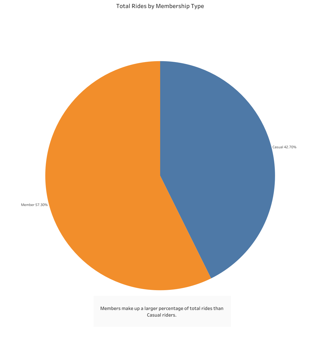
First up I create a visualization that shows the percentage of total rides by membership type. This is pretty straightforward, members make up a larger percentage of total rides than casual riders.

Next, let’s have a look at average ride time by each membership type:

Now we are beginning to see some difference in use: casual riders’ rides are nearly twice as long, on average, than members. Such a difference in ride time suggests completely different uses of the service. I want to look at the most used stations for each member type to see where they are coming and going from:

The most popular Casual rides begin and end near popular tourist attractions in the Downtown and Lake Shore areas of Chicago. The most popular stations for Member riders seem to coincide with bus stops near Metro stops and in areas with more office buildings than tourism interests. It appears that the casual riders are predominantly using the bikes for tourism and the member riders are using the service as a public transportation alternative for the daily needs of city life. I wonder if there are members using the service for tourism on the weekends, so I also compiled the top member weekend stations, they are almost the exact same as during the week with the exception of more difficult to reach leisure locations favored by locals, such as Theater on the Lake.

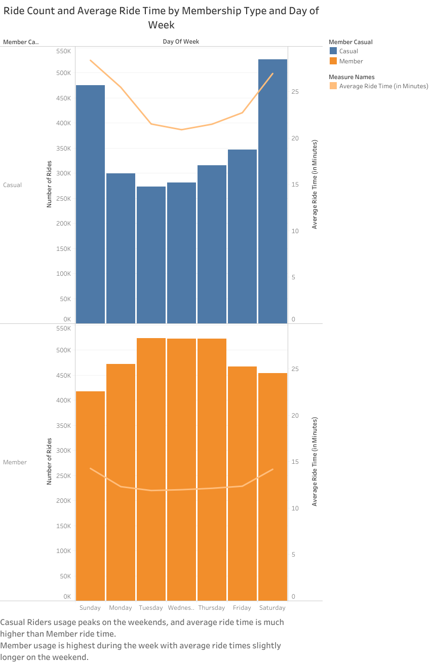
Looking at the total rides by day of week and membership type, casual rides peak on the weekends and member rides are higher during the week.

Looking at Monthly rides by member type, usage is much lower during the very cold Chicago winter, although for members it is much more constant throughout the warmer months, whereas Casual riders’ are much higher in the summer months when Chicago tourism is also highest.

Finally, looking at the Ride Count and Average Ride Time graph, Casual riders’ ride times and usage are both highest during the weekend, and while Member ride time does increase slightly on weekends it is still much shorter than Casual riders.

All of these findings make it clear that the two groups of Cyclistic clients use the ride share in fundamentally different ways, members for functional uses of daily life in Chicago, and Casual riders for tourism purposes.

Phase 6: Act

Findings and Recommendations: